This blog post is the second of a three-part series on NVIDIA's RAPIDS ecosystem. This post will address the potential performance benefits - along with more advanced use cases - of this innovative suite of libraries. In our final post, we will look at a real-world example and develop an end-to-end pipeline to apply an advanced Machine Learning use case.

When discussing GPU-accelerated computing, one of the most commonly mentioned points is the potential performance benefits that it can offer. NVIDIA state that when analysing datasets in the range of 10TB, RAPIDS can perform up to 20 times faster on GPUs than the top CPU baseline. Our team was curious to see whether RAPIDS could provide similar performance benefits on datasets of a somewhat smaller scale. 

Project Goals

The team set out to investigate the performance benefits of RAPIDS on GPUs, by carrying out a number of experiments, assessing the time taken to build and test three different models. For these experiments we chose to first build a K-means clustering model, followed by a random forest classifier, and then used VLAD encoding with the K-means algorithm for image clustering.

Our first two experiments used randomly generated data, while the third used a dataset of images of famous international tourist sites. We carried out our initial experiments with different dataset sizes, ranging from just 100 rows and 5,000 data points to 10 million rows and 500 million data points. For our third experiment, we used an image dataset which contained approximately 2GB of images.

As we use a range of dataset sizes for our first two experiments, showing a significant performance increase here would highlight that RAPIDS can offer performance benefits across a broad spectrum of datasets and use cases. In this blog post we will also mention the lower limits of these performance benefits and discuss where GPUs fail to produce better results.

The high-level results of our investigation can be found in the following table:

 

Compute	Spec	Price	K-Means Clustering	Random Forest Classifier	VLAD Encoding (w/ K-Means Clustering)
CPU	Intel Xeon (2.30GHz) (1 Core, 2 Threads)	~$200	RAPIDS is up to 24x faster	RAPIDS is up to 174x faster	RAPIDS is over 50x faster
GPU	NVIDIA T4 (2560 Cores)	~$1200

 

We used free Google Colab notebooks for the experiments in this blog.

Please read on to learn more!

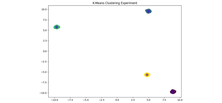
K-Means Clustering

We first import the required libraries and prepare to generate sample data using the make_blobs function from cuML.  We will vary the number of samples (n_samples) to assess how the performance benefits of cuML over Scikit-learn vary for different dataset sizes.

import cudf
import cupy
import numpy as np
import pandas as pd

import matplotlib.pyplot as plt

from cuml.datasets import make_blobs
from cuml.cluster import KMeans as cuKMeans

from sklearn.cluster import KMeans as skKMeans

%matplotlib inline

Figure 1. Import Libraries

 

We will begin our analysis with just 10,000 samples, and increase the sample size in subsequent experiments. We create a dataset with 50 features and 4 clusters, as shown in the code sample in figure 2.

n_samples = 10000
n_features = 50
n_clusters = 4

cu_data, cu_labels = make_blobs(
    n_samples=n_samples,
    n_features=n_features,
    centers=n_clusters,
    cluster_std=0.1
)

Figure 2. Creating Sample Data

 

We convert the sample data to Numpy arrays before first carrying out the K-means clustering using Scikit-learn. We use the timeit function to measure the execution time when clustering. This function runs the code a number of times and calculates the average execution time, along with the standard deviation. This code can be seen in figure 3 below.

np_data = cu_data.get()
np_labels = cu_labels.get()

kmeans_sk = skKMeans(
    init="k-means++",
    n_clusters=n_clusters,
    n_init = 'auto'
)
%timeit kmeans_sk.fit(np_data)

Figure 3. SciKit-Learn K-Means Clustering

 

We then carried out the same clustering with cuML, and once again calculated the average execution time and standard deviation. We repeated this experiment with datasets of various sizes, from 10 million rows to just 100 rows. We recorded the runtime when using Scikit-learn and when using cuML, and compared the two. The results can be found in the following table.

 

Rows	Data Points	Sklearn Runtime	cuML Runtime	Result
10,000,000	500,000,000	31.9 s ± 5.83 s	1.34 s ± 1.99 ms	~24x faster
1,000,000	50,000,000	1.58 s ± 383 ms	137 ms ± 2.8 ms	~11.5x faster
100,000	5,000,000	163 ms ± 11.6 ms	17.7 ms ± 636 µs	~9x faster
10,000	500,000	65.8 ms ± 11.5 ms	9.59 ms ± 730 µs	~7x faster
1000	50,000	22.6 ms ± 16.8 ms	14.8 ms ± 6.23 ms	~1.5x faster*
100	5000	1.94 ms ± 67.9 µs	4.48 ms ± 68.6	~2.3x slower

 

We can see that cuML is faster in nearly all cases, apart from the smallest dataset. The performance benefits of cuML seem to increase as dataset size increases. When using the dataset with 10 thousand rows, cuML is approximately seven times faster. When using the dataset with 10 million rows it is 24 times faster, a very significant improvement.

Figure 4. K-Means Clustering Results

 

Random Forest Classification

As with the K-means clustering experiment, we first imported the required libraries and set up the dataset. We varied the number of samples by increasing or decreasing the n_samples variable. We used scikit-learn’s make_classification function to generate random data that would be suitable for the experiment. We kept the total number of features, and the number of ‘useful’ features consistent for each attempt, and only varied the number of rows. We then split the dataset into training and testing subsets using scikit-learn’s train_test_split function. The code for importing libraries and setting up our data can be found in figure 5 below.

import cudf
import numpy as np
import pandas as pd

from cuml.ensemble import RandomForestClassifier as cuRFC
from cuml.metrics import accuracy_score

from sklearn.ensemble import RandomForestClassifier as skRFC
from sklearn.datasets import make_classification
from sklearn.model_selection import train_test_split

from sklearn.metrics import adjusted_rand_score

n_samples = 500000
n_features = 200 # total no. dimensions
n_info = 100 # no. useful dimensions
dtype = np.float32


x, y = make_classification(n_samples = n_samples,
                           n_features = n_features,
                           n_informative = n_info,
                           n_classes = 2)

x = pd.DataFrame(x.astype(dtype))
y = pd.Series(y.astype(np.int32))

x_train, x_test, y_train, y_test = train_test_split(x, y,
                                                    test_size = 0.2,
                                                    random_state=0)

Figure 5. Importing Libraries and Generating Data

 

For cuML modeling, we converted the data to cuDF datasets before model training. This can be seen in the code snippet in figure 6.

x_cuDF_train = cudf.DataFrame.from_pandas(x_train)
x_cuDF_test = cudf.DataFrame.from_pandas(x_test)

y_cuDF_train = cudf.Series(y_train.values)

Figure 6. Converting to cuDF Dataframe

 

For the sake of brevity, we won’t discuss parameter tuning in this blog post. For each experiment, we used consistent parameters when training our models. We timed model training and subsequent prediction using the testing subset. The time taken to train our models is compared in the table below. Code for creating a Random Forest Classification model for both Scikit-learn and cuML can be found in figure 7.

 

Rows	Data Points	Scikit-learn Runtime	Accuracy Score	cuML Runtime	Accuracy Score	Result
100,000	5,000,000	13min 25s	0.89	4.65 s	0.9	~174x faster
10,000	500,000	1min	0.86	523ms	0.85	~115x faster
1000	50,000	4.48s	0.67	550 ms	0.65	~8x faster*

 

As in the K-means clustering experiment, we found significant improvements when using cuML. Once again, these improvements were more pronounced for larger dataset sizes, and for our smaller datasets we saw that cuML offered less improvement.

#SK-learn model
sk_model = skRFC(n_estimators=40,
                 max_depth=16,
                 max_features=1.0,
                 random_state=10)

sk_model.fit(x_train, y_train)

#cuML model
cuml_model = cuRFC(n_estimators=40,
                   max_depth=16,
                   max_features=1.0,
                   random_state=10)

cuml_model.fit(x_cuDF_train, y_cuDF_train)

Figure 7. RFC Modelling

 

VLAD – Vector of Locally Aggregated Descriptors

For our third experiment we used VLAD encoding in a problem known as Content-Based Image Retrieval, which can be described as follows: “Given a query image, try to find visually similar images from an image database.”

In general, the workflow for content-based image retrieval is as follows:

• Take a database of images
• Take a query image.
• Search for the n most similar images in the database.

In practice, each image is usually stored as some form of embedding, which is a vector designed to capture the discriminative characteristics of the image. The discriminative characteristics are calculated by image descriptors, which are divided into two kinds: local image descriptors, and global image descriptors. Local image descriptors capture local information and spatial information (i.e. which features are present and how they are arranged with respect to one another) whereas global image descriptors only capture local information (i.e. which features are present). Global image descriptors work best when you want to capture certain features, regardless of their position in the image. In this case, the image dataset we are working with consists of photographs taken of famous tourist sites from various positions and angles. For this reason, global image descriptors are the most appropriate choice.

Workflow

The steps carried out in this experiment are as follows:

1. Calculate a Local Image Descriptor for all images in the database.
2. Cluster them into k-visual words.
3. Vectorise the whose database.

For a given query image, the retrieval workflow is then as follows:

4. Vectorize the image.
5. Perform vector retrieval.

The bulk of the implementation is contained within (3) and (4), which can be explained as follows:

• Given a vocabulary C={c1, c2, …, ck}     
• An image would be defined as v={v1, v2, …, vk}
• Where each visual work component is defined as:

 

 

Where:

• x: a local image feature.
• c_i: a vector describing the i^th visual word.
• NN(x): the nearest neighbour of x.

v  is then L2-normalised:  

 

 

Implementation and Results

The full python implementation is given in the appendix the end of this blog post. Our implementation makes use of Scikit-learn’s K-means, numpy’s algebraic calculation and opencv’s SIFT. After carrying out the workflow described above using this implementation, we then imported cuML’s K-means function and used this to replace the function from scikit-learn. This simple replacement provided a very significant improvement in performance. Clustering time decreased from 1620 seconds to just 28 seconds, making cuML’s clustering function over 50 times faster in this case. In this case, we carried out our experiment with a dataset of a fixed size, however, as we have once again used K-means clustering we can assume that the performance benefits will likely be greater with larger dataset sizes.

Replace:
    from sklearn.cluster import KMeans
    self.vocabs = KMeans(n_clusters = self.n_vocabs, init='k-means++').fit(X)
With: 
    from cuml.cluster import KMeans
    self.vocabs = KMeans(n_clusters = self.n_vocabs, init='k-means||').fit(X)

Figure 8. Replacing scikit-learn Clustering with cuML

 

A sample from the results of the image retrieval can be seen in figure 9 below. We have highlighted the query image with a blue border, and the resulting image set that is retrieved with a purple border.

Figure 9. Image Results

 

Conclusion

For all three experiments in this blog post we found that, once the dataset exceeded a minimum size, cuML provided significant performance benefits over Scikit-learn. These performance benefits are due to the use of GPU and seem to increase in magnitude as dataset size increases. In each experiment, we found that the conversion from traditional CPU-based methods to cuML was trivial and required very little additional work. The process was largely the same and the conversion typically involved swapping out functions from Scikit-learn with functions from cuML. Overall, we saw performance improvements of up to 50 times faster than the original method. In our final blog post on NVIDIA RAPIDS we will implement a full machine learning pipeline with RAPIDS and once again investigate the performance benefits and complexity of doing so.

Appendix

conf={
   'SIFT': {
        'output': 'feats-SIFT',
        'preprocessing': {
            'grayscale': False,
            'resize_max': 1600,
            'resize_force': False,
        },
    },
}

class ImageDataset(torch.utils.data.Dataset):
  default_conf = {
      'globs': ['*.jpg', '*.png', '*.jpeg', '*.JPG', '*.PNG'],
      'grayscale': False,
      'interpolation': 'cv2_area'
  }
  def __init__(self, root, conf, paths = None):
    self.conf = conf = SimpleNamespace(**{**self.default_conf, **conf})
    self.root = root
    paths = []
    for g in conf.globs:
      paths += list(Path(root).glob('**/'+g))
    if len(paths) == 0:
      raise ValueError(f'Could not find any image in root: {root}.')
    paths = sorted(list(set(paths)))
    self.names = [i.relative_to(root).as_posix() for i in paths]
  
  def __getitem__(self, idx):
    name = self.names[idx]
    image = read_image(self.root/name)
    size = image.shape[:2][::-1]
    feature = compute_SIFT(image)
    data = {
        'image': image,
        'feature': feature
    }
    return data
  def __len__(self):
    return len(self.names)

class VLAD:
  """
    Parameters
    ------------------------------------------------------------------
    k: int, default = 128
      Dimension of each visual words (vector length of each visual words)
    n_vocabs: int, default = 16
      Number of visual words
      
    Attributes
    ------------------------------------------------------------------
    vocabs: sklearn.cluster.Kmeans(k)
      The visual word coordinate system
    centers: [n_vocabs, k] array
      the centroid of each visual words
  """
  def __init__(self, k=128, n_vocabs=16):
    self.n_vocabs = n_vocabs
    self.k = k
    self.vocabs = None
    self.centers = None

  def fit(self,
          conf,
          img_dir:Path, 
          out_path: Optional[Path] = None,
          overwrite:bool = False):
    """This function build a visual words dictionary and compute database VLADs,
    and export them into a h5 file in 'out_path'

    Args
    ----------------------------------------------------------------------------
    conf: local descripors configuration
    img_dir: database image directory
    out_path: 
    """
    start_time = time.time()
    #Setup dataset and output path
    dataset = ImageDataset(img_dir,conf)
    if out_path is None:
      out_path = Path(img_dir, conf['vlads']+'.h5')
    out_path.parent.mkdir(exist_ok=True, parents=True)

    features = [data['feature'] for data in dataset] 
    X = np.vstack(features) #stacking local descriptor
    del features #save RAM
    #find visual word dictionary
    cluster_time = time.time()
    self.vocabs = KMeans(n_clusters = self.n_vocabs, init='k-means++').fit(X)
    print('Clutering time is {} seconds'.format(time.time()-cluster_time)) 
    self.centers = self.vocabs.cluster_centers_ 
    del X #save RAM

    # self._save_vocabs(out_path.parent / 'vocabs.joblib')
    for i,data in enumerate(dataset):
      name = dataset.names[i]
      v = self._calculate_VLAD(data['feature'])
      with h5py.File(str(out_path), 'a', libver='latest') as fd:
        try:
          if name in fd:
            del fd[name]
          #each image is saved in a different group for later
          grp = fd.create_group(name) 
          grp.create_dataset('vlad', data=v) 
        except OSError as error:
          if 'No space left on device' in error.args[0]:
            del grp, fd[name]
          raise error
    print('Execution time is {} seconds'.format(time.time()-start_time))
    return self

  def query(self,
        query_dir: Path,
        vlad_features: Path, 
        out_path: Optional[Path] = None,
        n_result=10):
    #define output path
    if out_path is None:
      out_path = Path(query_dir, 'retrievals'+'.h5')
    out_path.parent.mkdir(exist_ok=True, parents=True)

    query_names = [str(ref.relative_to(query_dir)) for ref in query_dir.iterdir()]
    images = [read_image(query_dir/r) for r in query_names]
    query_vlads = np.zeros([len(images), self.n_vocabs*self.k])
    for i, img in enumerate(images):
      query_vlads[i] = self._calculate_VLAD(compute_SIFT(img))

    with h5py.File(str(vlad_features), 'r', libver = 'latest') as f:
      db_names = []
      db_vlads = np.zeros([len(f.keys()), self.n_vocabs*self.k])
      for i, key in enumerate(f.keys()):
        data = f[key]
        db_names.append(key)
        db_vlads[i]= data['vlad'][()]

    sim = np.einsum('id, jd -> ij', query_vlads, db_vlads) # can be switch out with ANN
    pairs = pairs_from_similarity_matrix(sim, n_result)
    pairs = [(query_names[i], db_names[j]) for i,j in pairs]
    retrieved_dict = {}

    for query_name, db_name in pairs:
      if query_name in retrieved_dict.keys():
        retrieved_dict[query_name].append(db_name)
      else:
        retrieved_dict[query_name] = [db_name]

    with h5py.File(str(out_path), 'a', libver='latest') as f:
      try:
        for k,v in retrieved_dict.items():
          if k in f:
            del f[k]
          f[k] =v
      except OSError as error:
        if 'No space left on device' in error.args[0]:
          pass
        raise error
    return self
    
  def _calculate_VLAD(self, img_des):
    v = np.zeros([self.n_vocabs, self.k])
    NNs = self.vocabs.predict(img_des)
    for i in range(self.n_vocabs):
      if np.sum(NNs==i)>0:
        v[i] = np.sum(img_des[NNs==i, :]-self.centers[i], axis=0)
    v = v.flatten()
    v = np.sign(v)*np.sqrt(np.abs(v)) #power norm
    v = v/np.sqrt(np.dot(v,v))        #L2 norm
    return v